![]()
Optimizing a quantum circuit with FunFact
Install package and obtain assets if running on Google Colab
try:
    import google.colab
    !pip install funfact
except:
    pass
Introduction
In this tutorial we use FunFact to formulate a tensor expression that we use to optimize the parameters of a quantum circuit. Quantum circuits form a model for quantum computation in which the computation is represented by a sequence of simpler quantum gates acting on the individual qubits in the system, typically just one or two qubits. As the overall evolution of a closed quantum system is unitary, both the circuit and the individual gates are unitary operators. The individual gates are combined along the space dimension by Kronecker products and in time dimension by matrix inner products. This property of the circuit model allows us to write a quantum circuit as a FunFact tensor expression with unitary penalties on the leaf tensors.
This problem is also known as the quantum circuit synthesis or quantum compilation problem and we will explore the use of FunFact for solving it. We'll be using the PyTorch backend.
%matplotlib inline
%config InlineBackend.figure_format='retina'
import numpy as np
import matplotlib.pyplot as plt
from mpl_toolkits.axes_grid1 import make_axes_locatable
import funfact as ff
from funfact.initializers import Normal
from funfact.loss import MSE
from funfact import active_backend as ab
ff.use('torch')
ab
<backend 'PyTorchBackend'>
ab.set_printoptions(precision=3, sci_mode=False, linewidth=320)
Target data
The matrix that we will optimize a circuit structure for is the 3 qubit ($2^3 \times 2^3$) DFT matrix. We start by generating the target matrix in PyTorch data format:
n = 3
QFT_matrix = ab.tensor(np.matrix(np.fft.fft(np.eye(2**n)) / np.sqrt(2**n)))
QFT_matrix
tensor([[ 0.354+0.000j,  0.354+0.000j,  0.354+0.000j,  0.354+0.000j,  0.354+0.000j,  0.354+0.000j,  0.354+0.000j,  0.354+0.000j],
        [ 0.354+0.000j,  0.250-0.250j,  0.000-0.354j, -0.250-0.250j, -0.354+0.000j, -0.250+0.250j,  0.000+0.354j,  0.250+0.250j],
        [ 0.354+0.000j,  0.000-0.354j, -0.354+0.000j,  0.000+0.354j,  0.354+0.000j,  0.000-0.354j, -0.354+0.000j,  0.000+0.354j],
        [ 0.354+0.000j, -0.250-0.250j,  0.000+0.354j,  0.250-0.250j, -0.354+0.000j,  0.250+0.250j,  0.000-0.354j, -0.250+0.250j],
        [ 0.354+0.000j, -0.354+0.000j,  0.354+0.000j, -0.354+0.000j,  0.354+0.000j, -0.354+0.000j,  0.354+0.000j, -0.354+0.000j],
        [ 0.354+0.000j, -0.250+0.250j,  0.000-0.354j,  0.250+0.250j, -0.354+0.000j,  0.250-0.250j,  0.000+0.354j, -0.250-0.250j],
        [ 0.354+0.000j,  0.000+0.354j, -0.354+0.000j,  0.000-0.354j,  0.354+0.000j,  0.000+0.354j, -0.354+0.000j,  0.000-0.354j],
        [ 0.354+0.000j,  0.250+0.250j,  0.000+0.354j, -0.250+0.250j, -0.354+0.000j, -0.250-0.250j,  0.000-0.354j,  0.250-0.250j]], dtype=torch.complex128)
It is well-known that the unitary DFT matrix can be decomposed in a quantum circuit with $\mathcal{O}(n^2)$ one- and two-qubit gates. This implementation is also known as the Quantum Fourier Transform (QFT). The theoretical circuit structure is as follows:
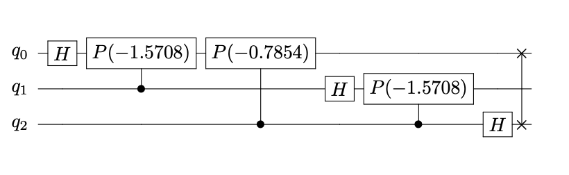
This circuit consists of:
- Hadamard gates:
- (Controlled) phase gates:
- SWAP gates.
A particular challenge that can prohibit runnig this circuit on quantum hardware is that the controlled phase gates and SWAP gates require an all-to-all connectivity between the qubits of the quantum computer. This connectivity is often available due to hardware constraints. Our goal is to recompile the QFT_matrix unitary into a circuit that can be implemented on a quantum device with linear connectivity between the qubits. To this end we define a function that generates a tensor expression for a two-qubit gate.
Quantum gates as tensor expressions
As an initializer for our two-qubit gates, we use the standard normal distribution. The unitary penalty is enforced by a unitary condition that is summed over the matrix elements of the leafs:
init = ff.initializers.Normal(std=1.0, dtype=ab.complex64)
unitary_cond = ff.conditions.Unitary(reduction='sum')
Next, we define a tensor expression for a two qubit gate acting on consecutive qubits $i, i+1$ of an $n$ qubit system.
def two_qubit_gate(i: int, n: int):
    ''' Generate a tensor expression that implements a two-qubit
    quantum gate acting on qubits i, i+1.

    Args:
        i (int): index of first qubit of two-qubit gate,
                 between 0 and n-2.
        n (int): total number of qubits.
    Returns:
        tsrex: tensor expression representing a two-qubit
        gate acting on qubits i, i+1 of an n-qubit system.

            ---
       i --|   |--
           | U |
     i+1 --|   |--
            ---

    '''
    G = ff.tensor(4, 4, initializer=init, prefer=unitary_cond)
    if i > 0 and i < n-2:
        tsrex = ff.eye(2**i) & G & ff.eye(2**(n-i-2))
    elif i == 0:
        tsrex = G & ff.eye(2**(n-2))
    elif i == n-2:
        tsrex = ff.eye(2**(n-2)) & G
    else:
        raise IndexError(f'Index i needs to satisfy: 0 <= i < {n-1}, got i={i}.')
    return tsrex
A two-qubit gate is thus represented as a Kronecker product of an (optimizibable) $4 \times 4$ matrix with unitary penalty and identity matrices that scale it up to an n-qubit matrix:
two_qubit_gate(1,4)
Quantum circuits from gates
Next, we generate the tensor expression for the complete circuit as a product of 3 two-qubit gates that are placed in a staggered pattern:
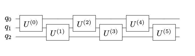
As time flows from left to right in a quantum circuit, the order in which the gates appears in a sequence of matrix multiplications is reversed compared to the circuit diagram:
circuit = two_qubit_gate(0, 3) @ \
          two_qubit_gate(1, 3) @ \
          two_qubit_gate(0, 3)
The loss function is the MSE-L2 loss, summed over the matrix elements:
MSE_loss = MSE('sum')
Next, we use the factorize method to opitimze the circuit tensor expression for the QFT_matrix unitary matrix:
circuit_fac = ff.factorize(
    circuit, QFT_matrix,
    max_steps=1000,
    tol=1e-3,
    lr=7e-2,
    vec_size=32,
    loss=MSE_loss,
    dtype=ab.complex64,
    checkpoint_freq=40,
    penalty_weight=2.0
)
28%|██▊ | 280/1000 [00:02<00:07, 97.39it/s]
The loss and total penalty on the circuit_fac factorization is:
print(f'loss: {MSE_loss(circuit_fac(), QFT_matrix)}')
print(f'penalty: {circuit_fac.penalty(sum_leafs=True)}')
loss: 0.00010626781269008971
penalty: 2.0135496470174985e-06
The penalties on the 6 individual leaf tensors are:
print(f'penalties: {circuit_fac.penalty(sum_leafs=False)}')
penalties: tensor([ 0.000, 0.000, 0.000])
A visual representation of the magnitude and phases of the QFT matrix and the optimized circuit model are shown below:
fig, axs = plt.subplots(2, 2, figsize=(8,6), dpi=200)
plt.subplots_adjust(hspace=0.3)

for ax, title, mat, vrange in [
    (axs[0, 0], 'Re(QFT)', ab.real(QFT_matrix), (0, 1)),
    (axs[0, 1], 'Im(QFT)', ab.imag(QFT_matrix), (-5, 5)),
    (axs[1, 0], 'Re(Circuit)', ab.real(circuit_fac()), (0, 1)),
    (axs[1, 1], 'Im(Circuit)', ab.imag(circuit_fac()), (-5, 5)),
]:
    ax.set_title(title)
    im = ax.matshow(mat, vmin=vrange[0], vmax=vrange[1], cmap='hot')
    divider = make_axes_locatable(ax)
    cax = divider.append_axes("right", size="5%", pad=0.1)
    plt.colorbar(im, cax=cax)

plt.show()

The unitarniness of the leaf tensors is visualized by plotting $|U^{(i)\dagger} U^{(i)}|$:
fig, axs = plt.subplots(1, len(circuit_fac.factors),
                        figsize=(15, 3), facecolor='w', edgecolor='k')
fig.subplots_adjust(hspace = .5, wspace=.001)

axs = axs.ravel()

for i, f in enumerate(circuit_fac.factors):
    data = ab.matmul(f, ab.conj(ab.transpose(f, (1, 0))))
    axs[i].matshow(ab.abs(data),vmin=0, vmax=1.0, cmap='hot')
    axs[i].set_title(f'factor {i}')
fig.suptitle('Unitariness of factor matrices: $|U^{\dagger}U|$', fontsize=18)
fig.tight_layout()
plt.show()

These $4 \times 4$ leaf tensors can be directly synthesized into native gates by means of direct methods such as the KAK decomposition.